Reproducing HERA Memo 4

In this demo, we are going to reproduce the results of Pober2015, a memo which estimated the sensitivity of the HERA array in its ultimate configuration. This memo was based on Pober+2014, which looked at the sensitivity of a “concept HERA” (which differs somewhat from the final instrument), as well as a few other well-known arrays.

The purpose of the demo is firstly to show how to estimate the sensitivity of a realistic array in a realistic situation. Secondly, it is a regression test, to ensure that the results given by the new code are consistent with the original code used in that memo.

The “reproduction” here is not expected to be exact – there are several small tweaks made in the current version that are not present in the code used for the memo (not to mention the code used for Pober+2014, which was not released at the time), for example cosmological calculations are done with astropy instead of approximate fitting functions. Nevertheless, we expect reasonable consistency when the settings are tuned to match the original code.

A Note On The Source Data

The data to which we compare in this notebook is precisely that used in Pober15. In that memo, the thermal noise estimates are not presented directly (either as a table or in plots), and only the ultimate SNR of the entire dataset is shown. We sourced the data for this notebook by installing and running the original code used for the memo with identical settings to those presented in the memo. This cannot be repeated easily since the original code requires Python <= 2. We include the resulting thermal sensitivities in this repo for posterity.

import py21cmsense as p21c
from astropy import units as un
from astropy.cosmology.units import littleh
from astropy.cosmology import Planck15
from astropy import constants
import matplotlib.pyplot as plt
import numpy as np

Original Data

memo_data = np.load(p21c.data.PATH / 'hera331drift_mod_0.135.npz')

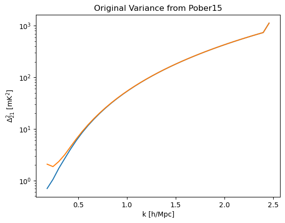
plt.plot(memo_data['ks'], memo_data['T_errs'], label='Thermal Variance')
plt.plot(memo_data['ks'], memo_data['errs'], label='Sample+Thermal Variance')
plt.yscale("log")
plt.title("Original Variance from Pober15")
plt.ylabel(r"$\Delta^2_{21}$ [mK$^2$]")
plt.xlabel("k [h/Mpc]");

HERA

P15 used a concept version of HERA that was a perfect hexagon (with no split-core), with 331 elements and no outriggers. It also used an approximation for the separation between hexagon rows of 12.12 m, which is close (but not exactly) the same as \(14.0 \sqrt{3}/2\). Let’s create such an array:

hera_ants = p21c.antpos.hera(hex_num=11, row_separation=12.12*un.m)

assert hera_ants.shape == (331, 3)

We will reproduce the results at \(\nu=135\) MHz (the default case in P15). Like P15, we use a dish size of 7 wavelengths at 150 MHz, which is close to, but not exactly, 14 m:

beam = p21c.GaussianBeam(frequency=135*un.MHz, dish_size=7 * (constants.c / (150 * un.MHz)).to("m"))

beam.dish_size

$13.990315 \; \mathrm{m}$

Now, let’s create the HERA Observatory model. Here, we set the receiver temperature to 100K, as per Table 1 of P14. We also set the latitude of the instrument to that of Green Bank (38:25:59.24), which was the assumed location of HERA in P14 & P15:

hera = p21c.Observatory(
    antpos=hera_ants,
    beam=beam,
    latitude=0.6707845*un.rad,
    Trcv=100*un.K,
)

Now, set up the observation itself. Here we assume a sky temperature model of \(60{\rm K} (\nu/300 {\rm MHz})^{-2.6}\), which is what P15 used (though there is no record of it in that memo, and this is slightly different from the sky model reference in Pober+14).

Furthermore, we set the number of days of observation to 180, with 6 hours per night, as described in that memo.

The coherent observation time in P15 is the “beam crossing time”, i.e. the size of the FWHM of the beam, at 150 MHz. In the modern version of the code, the observation duration is taken to be the FWHM at the observation frequency. For the sake of this comparison, we scale the observation duration back to the value at 150 MHz.

The integration time in 21cmSense plays a negligible role to first order: it controls how many times the UVWs are phased within the observation duration. The baselines are gridded in the UVW plane using a delta-function kernel (i.e. nearest-neighbours), and so changing the integration time merely changes how resolved their evolution across the UV-plane is. In the original 21cmSense, this value was hard-coded to 1 minute, so we set this value here.

Note: the phasing of UVWs has received a significant accuracy upgrade in the new 21cmSense, as we have moved to a pyuvdata-backed method. This will cause some small differences in the final sensitivity (sub-percent level).

Finally, as per S3.1.2 of P14, we use 8MHz of bandwidth, with 82 channels (providing ~0.1 MHz channel width).

obs = p21c.Observation(
    observatory=hera,
    tsky_amplitude=60*un.K,
    tsky_ref_freq=300*un.MHz,
    spectral_index=2.6,
    n_days=180,
    time_per_day=6*un.hour,
    bandwidth=8*un.MHz,
    n_channels=82,
    integration_time=60*un.s,
    lst_bin_size=beam.at(150*un.MHz).fwhm.value * 12/np.pi * 3600*un.s,
    use_approximate_cosmo=True,
    cosmo=Planck15.clone(H0=70.0, Om0=0.266)
)

obs.lst_bin_size.to(un.s)

$2077.3813 \; \mathrm{s}$

obs.uv_coverage.shape

finding redundancies: 100%|██████████| 330/330 [00:01<00:00, 303.03ants/s]
gridding baselines: 100%|██████████| 1260/1260 [00:00<00:00, 6204.30baselines/s]

(41, 41)

Now construct the sensitivity calculation. Here we use the “moderate” foreground model, with a horizon buffer of 0.1 h/Mpc, as mentioned in P15. The Legacy21cmFAST theory model is the same model used in the original code.

sense_moderate = p21c.PowerSpectrum(
    observation=obs,
    foreground_model='moderate',
    horizon_buffer=0.1 *littleh/un.Mpc,
    theory_model=p21c.theory.Legacy21cmFAST(),
)

sense1d = sense_moderate.calculate_sensitivity_1d(thermal=True, sample=True)
sense1d_t = sense_moderate.calculate_sensitivity_1d(thermal=True, sample=False)

calculating 2D sensitivity:   0%|          | 0/569 [00:00<?, ?uv-bins/s]calculating 2D sensitivity: 100%|██████████| 569/569 [00:01<00:00, 494.41uv-bins/s]
averaging to 1D: 100%|██████████| 159/159 [00:01<00:00, 141.53kperp-bins/s]
averaging to 1D: 100%|██████████| 159/159 [00:01<00:00, 132.20kperp-bins/s]

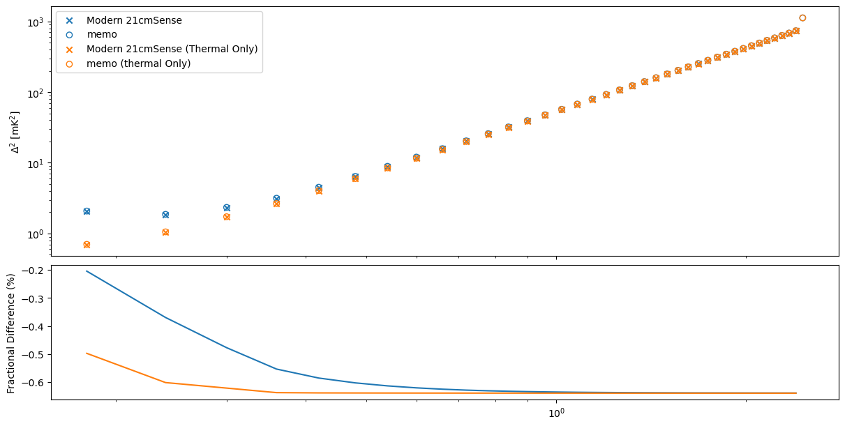
Plot the resulting comparison

fig, ax = plt.subplots(2, 1, sharex=True, figsize=(12, 6), constrained_layout=True, gridspec_kw={"height_ratios": [0.65, 0.35]})
ax[0].scatter(sense_moderate.k1d, sense1d, label='Modern 21cmSense', marker='x', color='C0')
ax[0].scatter(memo_data['ks'], memo_data['errs'], label='memo', color='C0', lw=1, facecolor='none')

ax[0].scatter(sense_moderate.k1d, sense1d_t, label='Modern 21cmSense (Thermal Only)', marker='x', color='C1')
ax[0].scatter(memo_data['ks'], memo_data['T_errs'], label='memo (thermal Only)', color='C1', facecolor='none')

ax[0].set_yscale("log")
ax[0].set_xscale('log')
ax[0].set_ylabel(r"$\Delta^2$ [mK$^2$]")
ax[1].set_ylabel("Fractional Difference (%)")
ax[1].plot(memo_data['ks'], 100*(sense1d[:len(memo_data['ks'])].value- memo_data['errs'])/memo_data['errs'])
ax[1].plot(memo_data['ks'], 100*(sense1d_t[:len(memo_data['ks'])].value- memo_data['T_errs'])/memo_data['T_errs'])
ax[0].legend();

/tmp/ipykernel_22655/2451292649.py:12: RuntimeWarning: invalid value encountered in subtract
  ax[1].plot(memo_data['ks'], 100*(sense1d[:len(memo_data['ks'])].value- memo_data['errs'])/memo_data['errs'])
/tmp/ipykernel_22655/2451292649.py:13: RuntimeWarning: invalid value encountered in subtract
  ax[1].plot(memo_data['ks'], 100*(sense1d_t[:len(memo_data['ks'])].value- memo_data['T_errs'])/memo_data['T_errs'])

Tests

The following are just assertions that the code reproduces the memo data within some tolerances, as can be seen already by the above plots. This is just for CI testing purposes.

mask = ~np.isinf(memo_data['errs'])

assert np.allclose(sense1d[:len(memo_data['ks'])][mask][:-1].value, memo_data['errs'][mask][:-1], rtol=1e-1)
assert np.allclose(sense1d_t[:len(memo_data['ks'])][mask][:-1].value, memo_data['T_errs'][mask][:-1], rtol=1e-2)