Getting Started

In this tutorial, you’ll learn the basics of using the py21cmsense library. See the README or the CLI-tutorial for information on the CLI interface.

import numpy as np
import matplotlib.pyplot as plt
from astropy import units as un
%matplotlib inline

from py21cmsense import GaussianBeam, Observatory, Observation, PowerSpectrum, hera

A Really Quick Demo

Let’s first just show how to go from nothing to a power spectrum sensitivity in a few lines. You’ll need the four main components of the sensitivity – a PrimaryBeam (in this case, the default GaussianBeam), an Observatory, an Observation and a Sensitivity (in this case, a PowerSpectrum one).

We can literally construct the whole thing at once:

sensitivity = PowerSpectrum(
    observation = Observation(
        observatory = Observatory(
            antpos = hera(hex_num=7, separation=14*un.m),
            beam = GaussianBeam(frequency=135.0*un.MHz, dish_size=14*un.m),
            latitude=38*un.deg
        )
    )
)

Warning

Note that this uses a default power spectrum from 21cmFAST defined at \(z=9.5\). It is up to you to use a different power spectrum if your observation redshift is different.

If all we care about is the 1D power spectrum sensitivity (including thermal noise and sample variance):

power_std = sensitivity.calculate_sensitivity_1d()

WARNING: AstropyDeprecationWarning: Transforming a frame instance to a frame class (as opposed to another frame instance) will not be supported in the future.  Either explicitly instantiate the target frame, or first convert the source frame instance to a `astropy.coordinates.SkyCoord` and use its `transform_to()` method. [astropy.coordinates.baseframe]
finding redundancies: 100%|██████████| 126/126 [00:00<00:00, 538.35ants/s]
computing UVWs: 100%|██████████| 39/39 [00:00<00:00, 122.86times/s]
gridding baselines: 100%|██████████| 468/468 [00:00<00:00, 10213.19baselines/s]
calculating 2D sensitivity: 100%|██████████| 216/216 [00:00<00:00, 327.98uv-bins/s]
averaging to 1D: 100%|██████████| 66/66 [00:00<00:00, 2807.86kperp-bins/s]

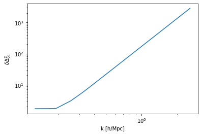
We can plot the sensitivity:

plt.plot(sensitivity.k1d, power_std)
plt.xlabel("k [h/Mpc]")
plt.ylabel(r'$\delta \Delta^2_{21}$')
plt.yscale('log')
plt.xscale('log')

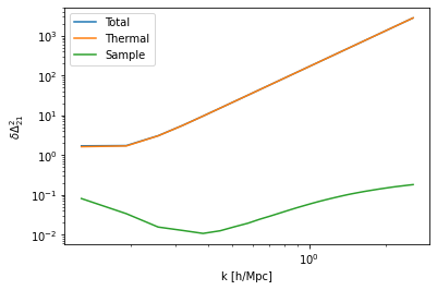
We could also have gotten the thermal-only and sample-only variance:

power_std_thermal = sensitivity.calculate_sensitivity_1d(thermal=True, sample=False)
power_std_sample = sensitivity.calculate_sensitivity_1d(thermal=False, sample=True)

averaging to 1D: 100%|██████████| 66/66 [00:00<00:00, 2698.27kperp-bins/s]
averaging to 1D: 100%|██████████| 66/66 [00:00<00:00, 2642.41kperp-bins/s]

plt.plot(sensitivity.k1d, power_std, label='Total')
plt.plot(sensitivity.k1d, power_std_thermal, label='Thermal')
plt.plot(sensitivity.k1d, power_std_sample, label='Sample')

plt.xlabel("k [h/Mpc]")
plt.ylabel(r'$\delta \Delta^2_{21}$')
plt.yscale('log')
plt.xscale('log')
plt.legend();

The Beam Object

Let’s go a bit more carefully and slowly through each of the components of the calculation. First we constructed a beam object. This can be directly accessed from our sensitivity:

beam = sensitivity.observation.observatory.beam

The beam houses attributes concerning the width and frequency-dependence of the beam. In practice, for the purpose of 21cmSense, it defines both the duration of an LST-bin (i.e. a set of times that for a given baseline can be coherently averaged) and the width of a UV cell (in the default settings, all baselines that fall into a given UV cell in a given LST bin are coherently averaged). It also defines the extent of the “wedge”.

Note that beam objects (and, indeed, all objects in 21cmSense) give all their outputs with astropy-based units. Here’s some examples:

beam.fwhm

$0.16774102 \; \mathrm{rad}$

beam.uv_resolution

6.304361399245074

beam.b_eff

$0.063589731 \; \mathrm{rad^{2}}$

Note that PrimaryBeam objects have attributes dependent on their frequency:

beam.frequency

$135 \; \mathrm{MHz}$

You can simply construct a new beam at a new frequency with the .at() method:

beam.at(160*un.MHz).b_eff/beam.b_eff

$0.71191406 \; \mathrm{}$

The Observatory

Next in the hierarchy of objects is the Observatory, which defines the attributes of the observatory itself. There are several options that can be given to its constructor, but it requires an array of antenna positions and a beam object (assumed to be the same for all antennas). You can view its documentation either with the help function, or at the online docs.

It also has some handy methods:

observatory = sensitivity.observation.observatory

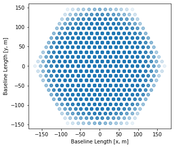
We can easily make a plot of the baseline positions:

plt.figure(figsize=(5,4.5))
plt.scatter(observatory.baselines_metres[:,:, 0], observatory.baselines_metres[:,:,1], alpha=0.1)
plt.xlabel("Baseline Length [x, m]")
plt.ylabel("Baseline Length [y, m]");

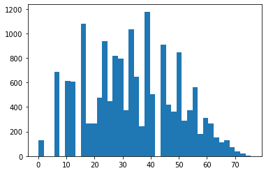
Or we can make a histogram of the baseline lengths (in wavelengths):

plt.hist(observatory.baseline_lengths.flatten(), bins=40);

The duration of an LST bin is also encoded in the observatory:

observatory.observation_duration.to("min")

$38.44341 \; \mathrm{min}$

The Observatory is in charge of the work of finding redundant baseline groups, as well as gridding the baselines (though these methods are called from the Observation itself):

red_bl = observatory.get_redundant_baselines()

WARNING: AstropyDeprecationWarning: Transforming a frame instance to a frame class (as opposed to another frame instance) will not be supported in the future.  Either explicitly instantiate the target frame, or first convert the source frame instance to a `astropy.coordinates.SkyCoord` and use its `transform_to()` method. [astropy.coordinates.baseframe]
finding redundancies: 100%|██████████| 126/126 [00:00<00:00, 817.13ants/s]

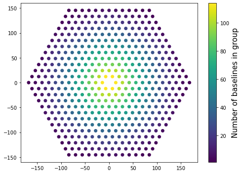
The output of this method is a little obfuscated, but it can be converted to something more easy to deal with:

baseline_group_coords = observatory.baseline_coords_from_groups(red_bl)
baseline_group_counts = observatory.baseline_weights_from_groups(red_bl)


plt.figure(figsize=(7,5))
plt.scatter(baseline_group_coords[:,0], baseline_group_coords[:,1], c=baseline_group_counts)
cbar = plt.colorbar();
cbar.set_label("Number of baselines in group", fontsize=15)
plt.tight_layout();

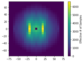
To grid the baselines, with rotation synthesis:

coherent_grid = observatory.grid_baselines(
    coherent=True,
    baselines=baseline_group_coords,
    weights=baseline_group_counts
)

computing UVWs: 100%|██████████| 39/39 [00:00<00:00, 117.02times/s]
gridding baselines: 100%|██████████| 468/468 [00:00<00:00, 11807.98baselines/s]

And we can view this grid:

plt.imshow(coherent_grid, extent=(observatory.ugrid().min(), observatory.ugrid().max())*2)
cbar = plt.colorbar()
cbar.set_label("Effective # of Samples")

The Observation

The Observation object has many more user-fed parameters – again, see them by using help(Observation), or by reading the online docs. Primarily, its job is to use these parameters to supply the Observatory methods with the parameters they need to derive their results.

observation = sensitivity.observation

For example, the baseline groups derived in the previous section show up as an attribute of the Observation:

plt.figure(figsize=(7,5))
x = [bl_group[0] for bl_group in observation.baseline_groups]
y = [bl_group[1] for bl_group in observation.baseline_groups]
c = [len(bls) for bls in observation.baseline_groups.values()]

plt.scatter(x, y, c=c)
cbar = plt.colorbar();
cbar.set_label("Number of baselines in group", fontsize=15)
plt.tight_layout();

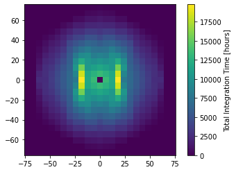
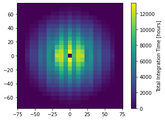
We can also get the total effective integration time spent in each UV cell (adjusting for coherent and incoherent averaging and all baselines):

plt.imshow(observation.total_integration_time.to("hour").value, extent=(observation.ugrid.min(), observation.ugrid.max())*2)
cbar = plt.colorbar()
cbar.set_label("Total Integration Time [hours]")

One nifty feature is that you can clone any of these objects, and replace certain attributes. So we can do:

observation_2 = observation.clone(coherent=False)

plt.imshow(observation_2.total_integration_time.to("hour").value,
           extent=(observation_2.ugrid.min(), observation_2.ugrid.max())*2)
cbar = plt.colorbar()
cbar.set_label("Total Integration Time [hours]")

finding redundancies: 100%|██████████| 126/126 [00:00<00:00, 812.29ants/s]
computing UVWs: 100%|██████████| 39/39 [00:00<00:00, 145.02times/s]
gridding baselines: 100%|██████████| 468/468 [00:00<00:00, 13602.11baselines/s]

Notice the reduction in effective integration time due to the assumption that different baseline groups cannot ever be averaged coherently.

Note also that these objects can be directly compared:

observation == observation_2

False

The Sensitivity

The design of 21cmSense is such that one might define sensitivity calculations for arbitrary statistical measurements from an interferometer. The default one that is implemented is the power spectrum (both 1D and 2D cylindrical).

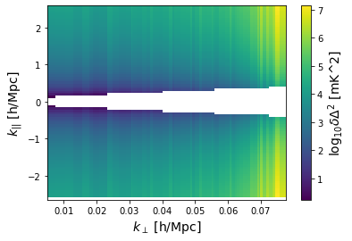
We have already shown some methods of the PowerSpectrum Sensitivity. It also has some helpful methods to calculate horizon lines etc. Let’s see what the 2D sensitivity looks like:

sense2d = sensitivity.calculate_sensitivity_2d()

The output here is a little strange – a dict of arrays. It can be used to make a 2D plot though:

sensitivity.plot_sense_2d(sense2d)

Conversely, we can calculate the 2D sensitivity on a grid of \(k_{\rm perp}, k_{||}\):

kperp = un.Quantity(np.linspace(0.01, 0.07, 15), 'littleh/Mpc')
kpar = un.Quantity( np.linspace(0.1, 2, 15), 'littleh/Mpc')
sense_gridded = sensitivity.calculate_sensitivity_2d_grid(kperp_edges=kperp, kpar_edges=kpar)

averaging to 2D grid: 100%|██████████| 66/66 [00:00<00:00, 4148.86kperp-bins/s]

plt.imshow(np.log10(sense_gridded.value.T), origin='lower')
plt.colorbar()

<matplotlib.colorbar.Colorbar at 0x7f5e1fb78fa0>

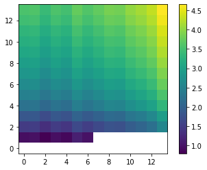
Notice the massive increase in sensitivity (lower values) because we binned in larger bins.

Excluding arbitrary k-bins

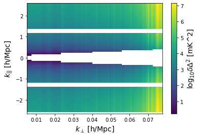
By default, the PowerSpectrum sensitivity class excludes modes in the wedge (plus some optional buffer) from contributing to the sensitivity. However, a particular experiment may have certain cylindrical \(k\) bins that are known to be affected by systematics (perhaps due to eg. cable reflections). You can ignore these modes by setting the systematics_mask parameter:

cable_refl_range = (un.Quantity(1.2, 'littleh/Mpc'), un.Quantity(1.4, 'littleh/Mpc'))
new_sense = sensitivity.clone(systematics_mask=lambda kperp, kpar: (np.abs(kpar) < cable_refl_range[0]) | (np.abs(kpar) > cable_refl_range[1]))

sense2d = new_sense.calculate_sensitivity_2d()
new_sense.plot_sense_2d(sense2d)

calculating 2D sensitivity: 100%|██████████| 216/216 [00:00<00:00, 386.70uv-bins/s]